2.2. Getting started
2.2.1. The derivative
How does numdifftools.Derivative work in action? A simple nonlinear function with a well known derivative is  . At
. At  , the derivative should be 1.
>>> import numpy as np
>>> from numpy import exp
>>> import numdifftools as nd
>>> f = nd.Derivative(exp, full_output=True)
>>> val, info = f(0)
>>> np.allclose(val, 1)
True
>>> np.allclose(info.error_estimate, 5.28466160e-14)
True
A second simple example comes from trig functions. The first four derivatives of the sine function, evaluated at , should be respectively ![[cos(0), -sin(0), -cos(0), sin(0)]](../_images/math/7f33d49c6cb4a6060d4fb6e95fbfcdac9e6f3a28.png) , or
, or ![[1,0,-1,0]](../_images/math/ce69ce94a2781aac46c883af901370d387421e32.png) .
.
>>> from numpy import sin
>>> import numdifftools as nd
>>> df = nd.Derivative(sin, n=1)
>>> np.allclose(df(0), 1.)
True
>>> ddf = nd.Derivative(sin, n=2)
>>> np.allclose(ddf(0), 0.)
True
>>> dddf = nd.Derivative(sin, n=3)
>>> np.allclose(dddf(0), -1.)
True
>>> ddddf = nd.Derivative(sin, n=4)
>>> np.allclose(ddddf(0), 0.)
True
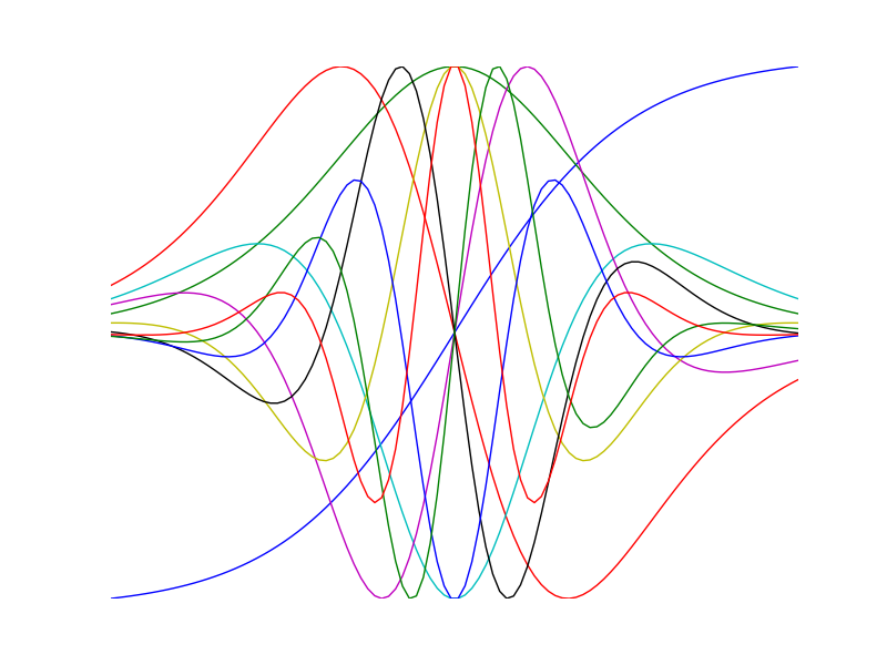
Visualize high order derivatives of the tanh function
>>> import numpy as np
>>> import matplotlib.pyplot as plt
>>> x = np.linspace(-2, 2, 100)
>>> for i in range(10):
...    df = nd.Derivative(np.tanh, n=i)
...    y = df(x)
...    h = plt.plot(x, y/np.abs(y).max())
plt.show()
2.2.2. Gradient and Hessian estimation
Estimation of the gradient vector (numdifftools.Gradient) of a function of multiple variables is a simple task, requiring merely repeated calls to numdifftools.Derivative. Likewise, the diagonal elements of the hessian matrix are merely pure second partial derivatives of a function. numdifftools.Hessdiag accomplishes this task, again calling numdifftools.Derivative multiple times. Efficient computation of the off-diagonal (mixed partial derivative) elements of the Hessian matrix uses a scheme much like that of numdifftools.Derivative, then Richardson extrapolation is used to improve a set of second order finite difference estimates of those mixed partials.
2.2.2.1. Multivariate calculus examples
Typical usage of the gradient and Hessian might be in optimization problems, where one might compare an analytically derived gradient for correctness, or use the Hessian matrix to compute confidence interval estimates on parameters in a maximum likelihood estimation.
2.2.2.2. Gradients and Hessians
>>> import numpy as np
>>> def rosen(x): return (1-x[0])**2 + 105.*(x[1]-x[0]**2)**2
- Gradient of the Rosenbrock function at [1,1], the global minimizer
>>> grad = nd.Gradient(rosen)([1, 1])
The gradient should be zero (within floating point noise)
>>> np.allclose(grad, 0)
True
- The Hessian matrix at the minimizer should be positive definite
>>> H = nd.Hessian(rosen)([1, 1])
The eigenvalues of H should be positive
>>> li, U = np.linalg.eig(H)
>>> [ bool(val>0) for val in li]
[True,  True]
- Gradient estimation of a function of 5 variables
>>> f = lambda x: np.sum(x**2)
>>> grad = nd.Gradient(f)(np.r_[1, 2, 3, 4, 5])
>>> np.allclose(grad, [  2.,   4.,   6.,   8.,  10.])
True
- Simple Hessian matrix of a problem with 3 independent variables
>>> f = lambda x: x[0] + x[1]**2 + x[2]**3
>>> H = nd.Hessian(f)([1, 2, 3])
>>> np.allclose(H, np.diag([0, 2, 18]))
True
- A semi-definite Hessian matrix
>>> H = nd.Hessian(lambda xy: np.cos(xy[0] - xy[1]))([0, 0])
one of these eigenvalues will be zero (approximately)
>>> [bool(abs(val) < 1e-12) for val in np.linalg.eig(H)[0]]
[True, False]
2.2.2.3. Directional derivatives
The directional derivative will be the dot product of the gradient with the (unit normalized) vector. This is of course possible to do with numdifftools and you could do it like this for the Rosenbrock function at the solution, x0 = [1,1]:
>>> v = np.r_[1, 2]/np.sqrt(5)
>>> x0 = [1, 1]
>>> directional_diff = np.dot(nd.Gradient(rosen)(x0), v)
This should be zero.
>>> np.allclose(directional_diff, 0)
True
Ok, its a trivial test case, but it easy to compute the directional derivative at other locations:
>>> v2 = np.r_[1, -1]/np.sqrt(2)
>>> x2 = [2, 3]
>>> directionaldiff = np.dot(nd.Gradient(rosen)(x2), v2)
>>> np.allclose(directionaldiff, 743.87633380824832)
True
There is a convenience function  that also takes care of the direction normalization:
>>> v = [1, -1]
>>> x0 = [2, 3]
>>> directional_diff = nd.directionaldiff(rosen, x0, v)
>>> np.allclose(directional_diff, 743.87633380824832)
True
2.2.2.4. Jacobian matrix
Jacobian matrix of a scalar function is just the gradient
>>> jac = nd.Jacobian(rosen)([2, 3])
>>> grad = nd.Gradient(rosen)([2, 3])
>>> np.allclose(jac, grad)
True
Jacobian matrix of a linear system will reduce to the design matrix
>>> A = np.random.rand(5,3)
>>> b = np.random.rand(5)
>>> fun = lambda x: np.dot(x, A.T) - b
>>> x = np.random.rand(3)
>>> jac = nd.Jacobian(fun)(x)
This should be essentially zero at any location x
>>> np.allclose(jac - A, 0)
True
The jacobian matrix of a nonlinear transformation of variables evaluated at some arbitrary location [-2, -3]
>>> fun = lambda xy: np.r_[xy[0]**2, np.cos(xy[0] - xy[1])]
>>> jac = nd.Jacobian(fun)([-2, -3])
>>> np.allclose(jac, [[-4.,  0.],
...                   [-0.84147098,  0.84147098]])
True
2.3. Conclusion
numdifftools.Derivative is an a adaptive scheme that can compute the derivative of arbitrary (well behaved) functions. It is reasonably fast as an adaptive method. Many options have been provided for the user who wishes the ultimate amount of control over the estimation.